Tracking Analysis Pattern Recognition

First, a calibration process was carried out to obtain slewing constants for the scintillator timing. Figure  shows the mean time vs pulse height for one of the hodoscopes. A polynomial is fitted to this distribution and used to correct the mean time.

  
Figure: Mean time vs. pulse height (arbitrary units) from scintillation counter simulation. The slewing which is clearly visible is corrected in the analysis.

The top and bottom photomultiplier times are used to calculate both the mean time and the time difference, which gives the vertical position. The pulse heights are used for the slewing correction and to calculate the geometric mean pulse height, which is normalized to minimum ionizing (charge 1) and then used to assign a charge to the particle causing the hit. The charges are assigned according to Table .

  
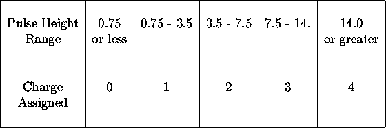
Table: Scintillator pulse height values used to assign charges in analyzing Monte Carlo data. Pulse heights are normalized to charge 1.

Pattern recognition then begins with the hodoscopes since, as discussed above, the hodoscopes provide a large amount of correlated information. For our Monte Carlo studies we reconstructed every track passing the cuts described below. In fact the only interesting tracks are those with velocities considerably less than the speed of light ( 0.973). In the analysis of data from the experiment we will impose time cuts on the hodoscope tracks before trying to fully reconstruct tracks. Since on average there are less than two tracks per event passing the ``late time'' cut, this will greatly reduce the computing time required for pattern recognition.

The pattern recognition proceeds by the following steps:

1. Find Hodoscope tracks. Find sets of hodoscope hits in H1,H2,H3 which have the same assigned charge, fit a line (within appropriate errors) in the horizontal, vertical and time dimensions. Cut on vertical and time projection to target.
2. Find confirming hits in all views in the downstream straw tube arrays (S2,S3).
3. Refit the horizontal and vertical track parameters using the straw tube information and cut again on the vertical projection to the target.
4. Do preliminary kinematics. Calculate rigidity from charge, angle and position of downstream track assuming the track emanated from the target. Project back upstream through second magnet (M2) and find confirming hit in all views in straw tube array S1.
5. Fit velocity and cut on 0.701 0.973 (covering the rapidity range of interest).
6. Calculate rigidity and mass. If the mass is greater than 1.5GeV/c , (i.e. not a proton or lighter particle) use the velocity and a mass of 0.938 (proton mass) to calculate a rigidity R . Use R to track the downstream track segment back through the second magnet to S1. If a confirming hit is found in S1 the candidate is considered ambiguous with a conventional explanation (proton track not from target interaction) and is rejected.

Figure  shows the number of reconstructed tracks found in the scintillator hodoscopes per event using the cuts described above. Figure  shows the number of tracks per event with confirming hits found in the downstream straw tube arrays, and Fig.  shows the number of tracks per event with confirming hits in the upstream straw tube array. The means are shown on each histogram. The similarity of the means indicates that tracks found in the scintillators have a high probability of being good tracks confirmed in the other detectors.

  
Figure: Reconstructed tracks found in the scintillator hodoscopes per event.

  
Figure: Number of tracks per event with confirming hits found in the downstream straw tube arrays.

  
Figure: Number of tracks per event with confirming hits in the upstream straw tube array.